The 2 Most Popular Graph Traversal Algorithms

Why are graph traversal algorithms so valuable? They visit every single connected node in the graph – that is, given a node, all the vertices connected to it. In this article, you will find out more about how the two most popular algorithms in this class actually work.

Graph Traversal Algorithms – Overview

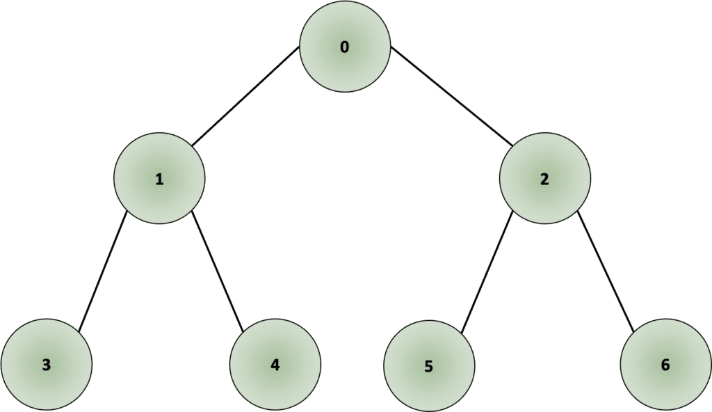
Visually a graph traversal is typically drawn as a decision tree, as shown in Fig. 1.

When traversing all the nodes through a graph, regardless of the algorithm used, we can face the following issues:

1. There may be cases in which the graph is not connected, therefore not all nodes can be reached.
2. In the case of cyclic (starts and ends at the same node) graphs, we should make sure that cycles do not cause the algorithm to go into an infinite loop.
3. We may need to visit some nodes more than once, since we do not know if a node has already been seen, before transitioning to it.

Graph traversal algorithms can solve the second and third problems by flagging vertices as visited when appropriate: (1) at first, no node is flagged as visited; (2) when the node is visited, we flag it as visited during the traversal; (3) a flagged node is not visited a second time. This keeps the program from going into an infinite loop when it encounters a cycle.

Traversing a graph is, without a doubt, one of the most useful processes when dealing with graphs. In this blog we will describe the two most frequent methods when traversing a graph:

• Depth first search (DFS)
• Breadth first search (BFS)

Depth First Search (DFS)

In this algorithm, we follow one path as far as it will go. The algorithm starts in an arbitrary node, called root node and explores as far as possible along each branch before backtracking.

The algorithm can also be applied to directed graphs. DFS is implemented with a recursive algorithm and its temporal complexity is O(E+V).

How does it work CONCEPTUALLY?

The DFS algorithm starts at the root (top) node of a tree and goes as far as it can down a given branch (path), then backtracks until it finds an unexplored path, and then explores it. The algorithm does this until the entire graph has been explored.

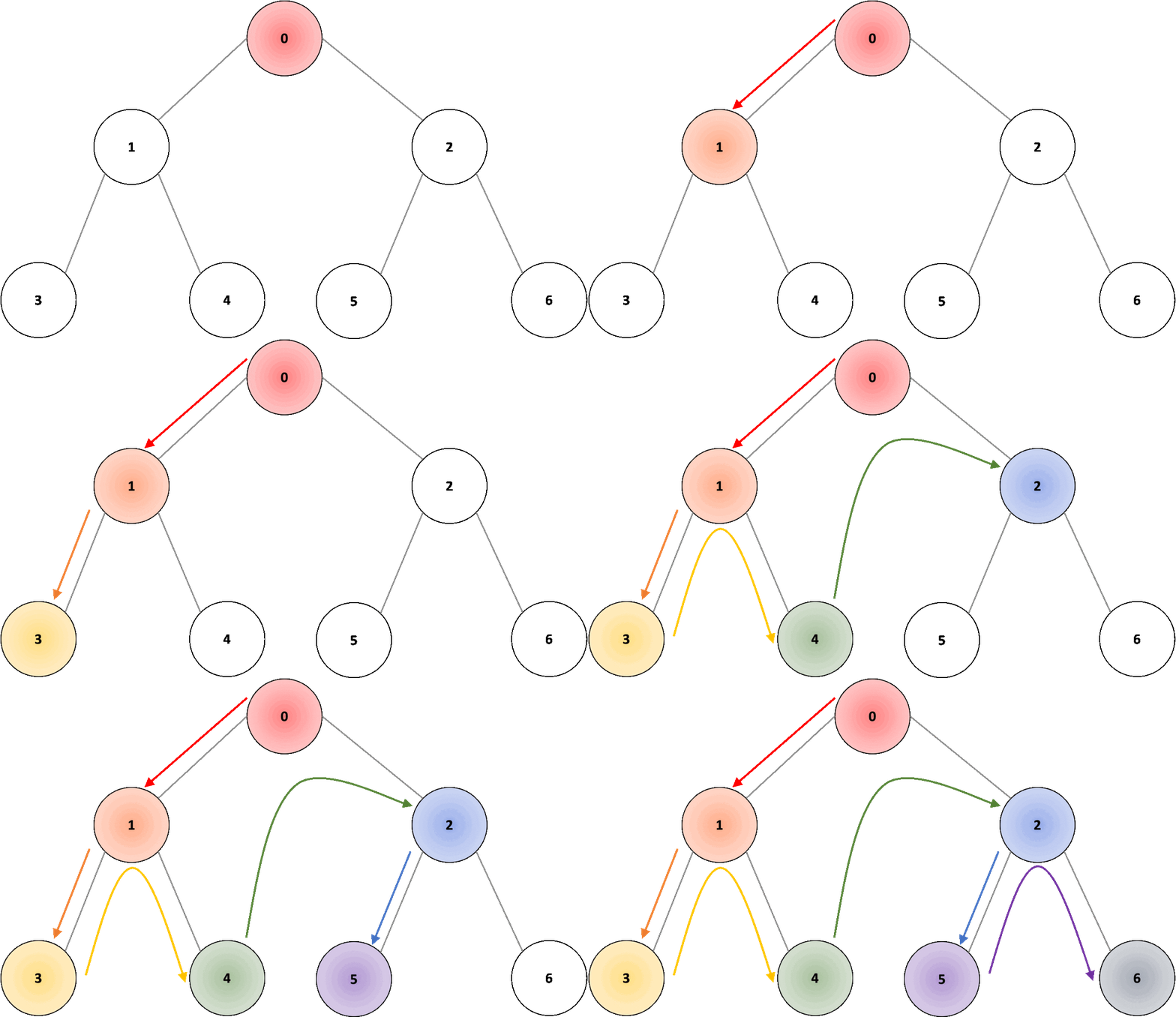
In the example shown in Fig. 2, the root node would be node “0”; we traverse in depth through node “1”, followed by node “3”. Once we reach the node, we move one level up to node “1” and traverse through all other connected nodes, in this case, node “4”. Once we have covered all connected nodes, we move again one level up, to node “0” and traverse all other connected nodes, in this case, node “2”. As we traverse through deeper nodes, we traverse through nodes “5” and “6”, covering all connected nodes.

Breadth First Search (BFS)

In the BFS algorithm, rather than proceeding recursively, we pull out the first element from the queue, check if it has a path, check if it is the destination node we are interested in and if not add all the children nodes to it. We look at all the nodes adjacent to one before moving on to the next level.

The algorithm can also be applied to directed graphs. The algorithm’s time complexity is O(E+V).

How does it work CONCEPTUALLY?

The BFS algorithm starts by searching a start node, followed by its adjacent nodes, then all nodes that can be reached by a path from the start node containing two edges, three edges, and so on.

In the example below from Fig. 3, the root node would be node “0”; we traverse in width through node “1”, followed by node “2”. Once we have traversed through all nodes in the first depth level, we move to the second depth level, starting with node “3”, and moving through nodes “4”, “5”, and “6”.

DFS vs. BFS

As discussed here, BFS is used to search nodes that are closer to the given source; while DFS is used instead in cases where the solution is away from the source.

When coming to practical examples, BFS is typically used to find the shortest distance between two nodes, such as routing for GPS navigation; while DFS is more suitable for e.g. game/puzzle problems: we make a decision, then explore all paths through this decision, and if this decision leads to a win situation, then we stop.

Traversal algorithms are also a fundamental component for numerous additionally complex graph algorithms. For instance, the DFS and BFS traversal algorithms often show up bundled into more advanced graph algorithms, such as:

• Shortest path in an unweighted graph
• Topological sorting
• Strongly connected component
• 2 Satisfaction (2-SAT)
• Lowest Common ancestor (LCA)
• Max Flow / Min Cut

Conclusions

As mentioned in the introduction, there are two main algorithms to traverse all nodes in a graph: (1) DFS, focusing on traversing nodes by depth, before moving to the next level nodes; and (2) BFS, focusing on traversing nodes by width within the same level, before moving to the next depth level in the graph. Both algorithms have the same temporal complexity and are easy to logically program.

As shown above, these traversal algorithms are the pillars of other graph algorithms, such as the shortest path algorithm. For instance, the Uber H3 article from Lead Data Scientist Sean Robinson, speaks about the geospatial distribution of bike stations in major cities, and it uses the unweighed shortest path algorithm to find the shortest path between two bike stations, which is based on BFS. For an introductory article on graph database geospatial analysis, follow the link.

In this blog, we covered the two most common algorithms to traverse all connected nodes in a graph, examined the mechanisms that differentiate these algorithms, and introduced practical use cases where they can be applied to deliver value. These two algorithms provide the opportunity to be applied in countless applications, many of which are waiting to be discovered.

These and other graph algorithms make up the tools by which modern machine learning is advancing, via graphs and graph data science.

Read Related Articles

• What is Graph Data Science?
• What is Neo4j Graph Data Science?
• What are Graph Algorithms?
• Pathfinding Algorithms (Top 5, with examples)
• Closeness Centrality
• Degree Centrality
• Betweenness Centrality
• PageRank
• Conductance Graph Community Detection: Python Examples
• Graph Embeddings (for more on graph embedding algorithms)
• LLM Pipelines / Graph Data Science Pipelines / Data Science Pipeline Steps

Also read this related article on graph analytics for more on analytics within the graph database context.