CONTACT US
Making the Most of the Betweenness Centrality Algorithm for Gaining Unique Insights

Betweenness Centrality is one of several of a category called ‘centrality algorithms’. Centrality algorithms are used to understand the roles of nodes in a graph and their impact on the network. It was initially centered on social network analysis and sociograms in the 1940s, to analyze social cliques. It was in 1948 that psychologist Alex Bavelas introduced this authentic concept for the first time as a mathematical model to study groups in social networks.
Centrality Algorithms and the Uniqueness of the Betweenness Centrality Algorithm
As mentioned above, the goal of centrality algorithms is to measure the importance of various nodes in a graph network, or in other words, how central a node is in a graph. (For more on graphs and graph databases, checkout our article on “What is a graph database?”.) The next logical question that emerges is: how do we define importance?
There are several centrality algorithms that focus on identifying the most important nodes in the network, based on the question we want to answer. The most common centrality algorithms are:
- Degree Centrality: used to find the individual nodes’ “popularity”, by looking into the number of incoming and outgoing relationships.
- Closeness Centrality: used to detect nodes that can spread information efficiently measuring how central a node is to the group.
- Betweenness Centrality: used to detect how influenceable a node is over the flow of information or resources in a graph.
- PageRank: used to measure the influence of nodes. This is also is the best-known of the centrality algorithms.
In this blog, we will focus on the Betweenness Centrality Algorithm. It is unique because it is typically used to find nodes that serve as a bridge from one part of a graph to another. It is a way of detecting the amount of influence a node has over the flow of information or resources in a graph. For example, it can be used to know which node in a funnel process is the busiest and, by evaluating these vulnerable nodes, make decisions on how to optimize the process.
We will examine how the algorithm works conceptually then look at a use case to have a better grasp of the algorithm’s uses, and then end by understanding it mathematically.
Betweenness Centrality Algorithm – Concept
The concept was originally introduced by J.M. Anthonisse (1971) and L. C. Freeman (1977); both are based on shortest-path distances. The algorithm uses Brandes’ approximate algorithm (Brandes & Pich, 2006) for unweighted graphs; while for weighted graphs it uses multiple concurrent Dijkstra algorithms (E. W. Dijkstra, 1959).
This algorithm was originally used in the social network and psychology fields, where the Betweenness Centrality Score identifies a person’s role in allowing information to pass from one part of the network to the other. As technology has evolved, and we have more and more access to the data and its interconnections, the use of the betweenness centrality algorithm has been extended into other cases such as transportation networks, epidemics, rumors, where we are interested in finding the bottleneck in a process or the most influential node in a network. We should always keep in mind that one of the challenges of this algorithm is the sparsity of the graph network.
Use case: Applying Betweenness Centrality to the Supply Chain Risk
A good use case of the Betweenness Centrality algorithm can be applied in the supply chain process, when transporting a product internationally from country A to country B by cargo ships, stopping in intermediate ports to replenish supplies. To avoid port congestion and find which port is the best connected, we create a Global Liner Shipping Network (GLSN) containing the main ports, connections among them and number of cargo ships at the dock and the port traffic capacity. Fig. 1 shows consisting of 977 nodes (i.e., ports) and 16,680 edges (i.e., inter-port links).
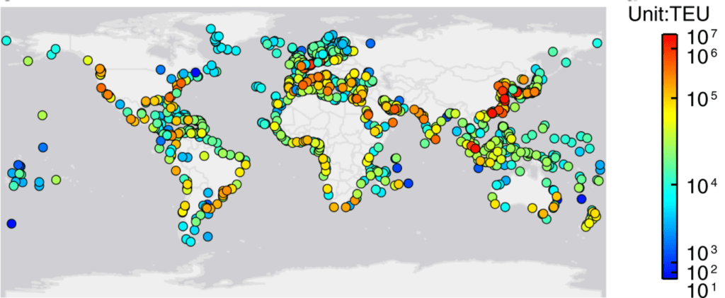 Fig. 1: Ports in the GLSN. The color of nodes corresponds to the traffic capacity of ports measured in Twenty-Foot Equivalent Unit (TEU). Source: T. LaRock, M. Xu & T. Eliassi-Rad (2022) Fig. 1: Ports in the GLSN. The color of nodes corresponds to the traffic capacity of ports measured in Twenty-Foot Equivalent Unit (TEU). Source: T. LaRock, M. Xu & T. Eliassi-Rad (2022) | 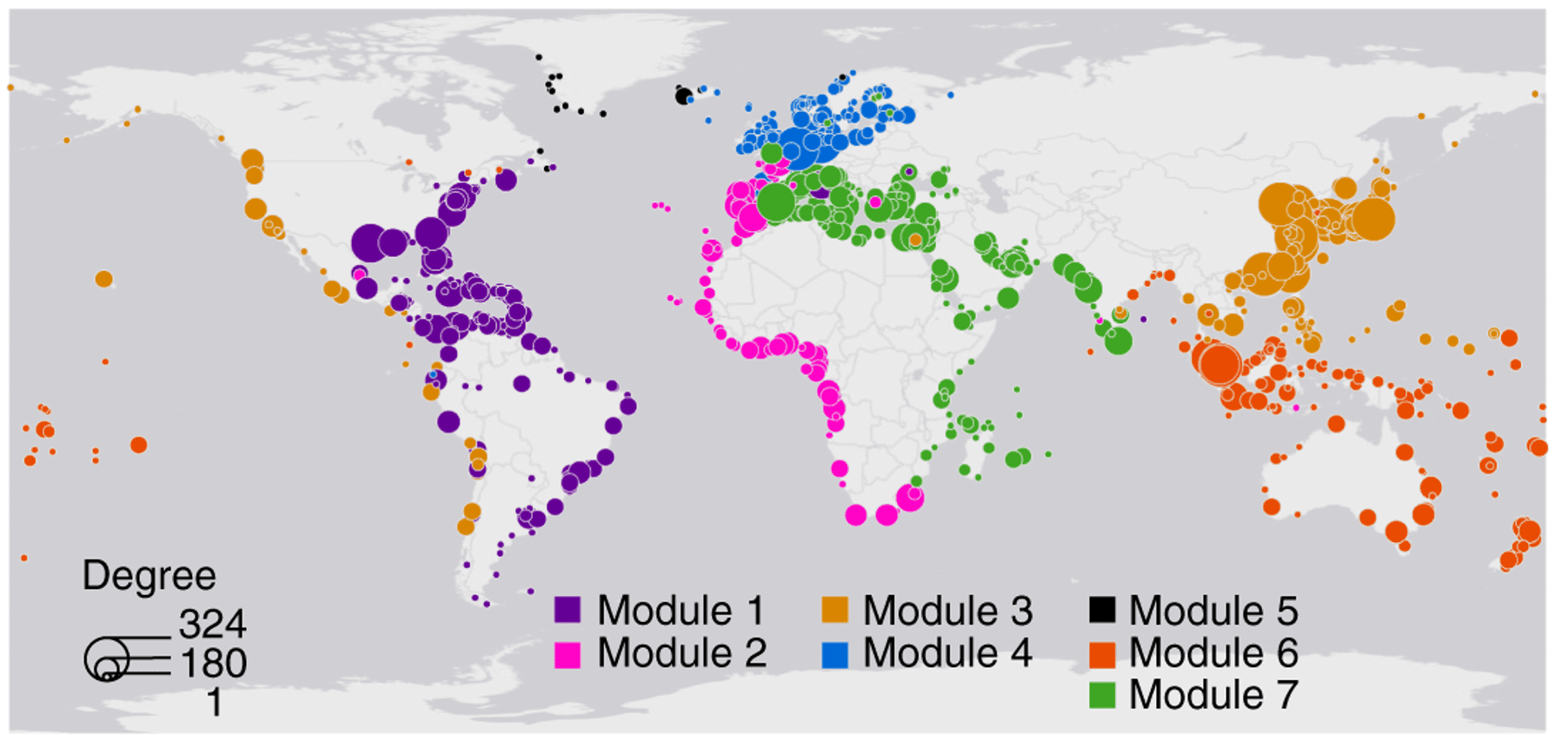 Fig. 2: Division of the port communities into large networks (7 different modules). Source: T. LaRock, M. Xu & T. Eliassi-Rad (2022) Fig. 2: Division of the port communities into large networks (7 different modules). Source: T. LaRock, M. Xu & T. Eliassi-Rad (2022) |
For simplicity purposes, we build a small version of the global liner shipping network, focusing on the modules shown in Fig. 2. The Betweenness Centrality Score will measure the importance of a port to the navigation of the system (e.g. LaRock, Xu & Eliassi-Rad, 2022) and will tell us which port is the most influential.
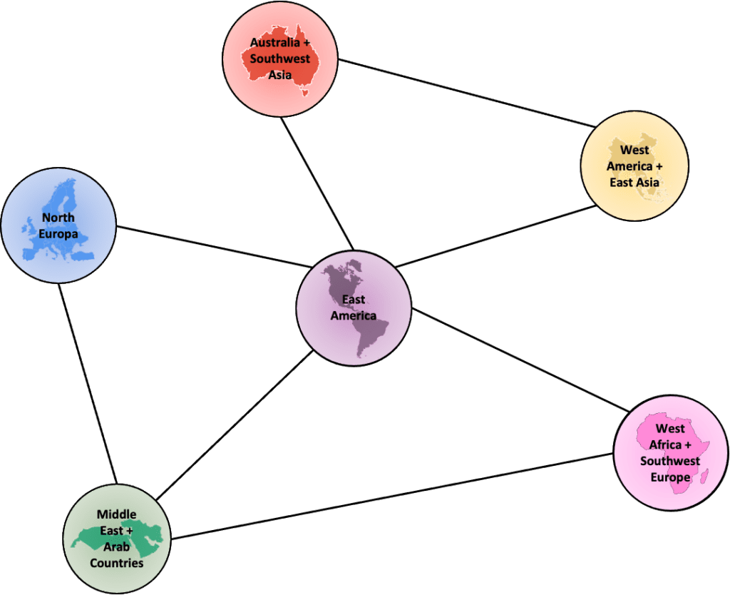
The simplistic example shown in Fig. 3 helps is visualizing how the ports (nodes) are interconnected between them (edges). Each node (port) would have port traffic capacity and the number of ships at a certain time as properties and would be connected.
To further illustrate the point, during the global supply chain shortage in 2021 we would have seen that major ports connecting Asia with North America, such as the one in Oakland, CA would have resulted in a high betweenness centrality score, as it was one of the bottleneck ports during this period.
Keeping this example in mind, let’s now take a look at the algorithm from the mathematical point of view to better understand what happens under the hood.
Mathematical Approach for the Betweenness Centrality Algorithm
The estimate of the betweenness centrality score can be explained with the following equation:

where u refers to a node; p is the total number of shortest paths between the nodes s and t, and p(u) is the number of shortest paths between the nodes s and t that pass-through node u.
Let’s focus on a more tangible description: taking a node u to analyze, we look at all the nodes not including the chosen node u; choose a pair of nodes to analyze (s, t).

For the pair (s=5; t=3) let’s divide the number of relationships that pass through the node u (1, in yellow) by the number of relationships between the two nodes s and t (2, in yellow and orange).
Repeating this process for all pairs of nodes in the graph, excluding the node u, we end up with the table below:
| Relationships that pass by node u P(u) in Eq. 1 | Total relationships between pairs of nodes u in Eq. 1 | Ratio B(u) in Eq. 1 |
| p1,2(6)=0 | u1,2(6)=1 | 0 |
| p1,3(6)=1 | u1,3(6)=1 | 1 |
| p1,4(6)=1 | u1,4(6)=1 | 1 |
| p1,5(6)=1 | u1,5(6)=1 | 1 |
| p2,3(6)=1 | u2,3(6)=1 | 1 |
| p2,4(6)=1 | u2,4(6)=1 | 1 |
| p2,5(6)=1 | u2,5(6)=1 | 1 |
| p3,4(6)=0 | u3,4(6)=1 | 0 |
| p3,5(6)=1 | u3,5(6)=2 | 0.5 |
| p4,5(6)=0 | u4,5(6)=1 | 0 |
The sum B(u)=6.5 is the betweenness centrality for the node u=6. However, the sum has not been normalized by the size of the network – it is not the same to have a betweenness sum of 6.5 in a 5-node graph than in a node in a 500-node graph. To normalize the betweenness score, we need to consider if the graph has directionality or not:
- To determine if the graph has directionality: we divide by the total number of pairs of nodes, not including the chosen node u, resulting in

which in this example above it would be (6-1)*(6-2)/2=10.
- The graph does not have directionality: the normalization term would be:

Betweenness Centrality Score = 1 represents the highest betweenness centrality, while Betweenness Centrality Score = 0 represents the lowest betweenness centrality. In our example, the betweenness centrality results in 0.65 for node 6.
Model Performance
While Betweenness Centrality offers unique insights to identify bottlenecks within a network, a common challenge many will face with this algorithm is the lack of scalability as the network size increases.
This algorithm is very resource-intensive to compute and running the algorithm on an undirected graph is about twice as computationally intensive compared to a directed graph.
The Brandes’ approximate algorithm for unweighted graphs used in Betweenness Centrality (see concept section) has a time complexity of O(nm + n2logn) and a space complexity of O(n + m), where n and m are the number of vertices and edges in a graph, respectively (see S. Bhardwaj, R. Niyogi & A. Milani, 2011 for more details). The Dijkstra algorithm in weighted graphs (see concept section) has a time complexity of O(n * m) instead (see here for more details), but we should keep in mind that Betweenness Centrality uses multiple concurrent Dijkstra algorithms.
Therefore, time complexity is something to take into account when working with large graph networks.
However many implementations of the algorithm offer a sampling mechanism to combat this inefficiency. Riondato & Kornaropoulos, 2016 developed an algorithm that uses a predetermined number of samples of node pairs k, reducing the time complexity and getting the same probabilistic on the quality of the approximation. In this case, the time complexity is reduced to O(k * m) where k is the number of samples used, and m is the number of edges.
Conclusion
Throughout this article we’ve seen how the Betweenness Centrality algorithm is used to identify which nodes form the strongest bottlenecks within a graph network. Based on this definition of importance, we can use this measure to detect bottlenecks in a variety of different use cases.
We have seen that, although the mathematical concept is not particularly complex, the algorithm’s computational complexity can create limitations for larger datasets if not accounted for through sampling. Despite this, Betweenness Centrality unfortunately can be somewhat of a ‘dark horse’ graph algorithm that can often be overlooked despite the unique insights it has to offer.
These and other graph algorithms make up the tools by which modern machine learning is advancing, via graphs and graph data science. If you are evaluating whether an AI project will be a fit, read about whether an AI consulting partner is right for you to help evaluate and deliver.
Read Related Articles
- What is Graph Data Science?
- What is Neo4j Graph Data Science?
- What are Graph Algorithms?
- Graph Traversal Algorithms (a.k.a Pathfinding algorithms)
- Pathfinding Algorithms (Top 5, with examples)
- Closeness Centrality
- Degree Centrality
- PageRank
- Conductance Graph Community Detection: Python Examples
- Graph Embeddings (for more on graph embedding algorithms)
Also read this related article on graph analytics for more on analytics within the graph database context.
Graphable helps you make sense of your data by delivering expert data analytics consulting, data engineering, custom dev and applied data science services.
We are known for operating ethically, communicating well, and delivering on-time. With hundreds of successful projects across most industries, we have deep expertise in Financial Services, Life Sciences, Security/Intelligence, Transportation/Logistics, HighTech, and many others.
Thriving in the most challenging data integration and data science contexts, Graphable drives your analytics, data engineering, custom dev and applied data science success. Contact us to learn more about how we can help, or book a demo today.
Still learning? Check out a few of our introductory articles to learn more:
- What is a Graph Database?
- What is Neo4j (Graph Database)?
- What Is Domo (Analytics)?
- What is Hume (GraphAware)?
Additional discovery:
- Hume consulting / Hume (GraphAware) Platform
- Neo4j consulting / Graph database
- Domo consulting / Analytics - BI
We would also be happy to learn more about your current project and share how we might be able to help. Schedule a consultation with us today. We can also discuss pricing on these initial calls, including Neo4j pricing and Domo pricing. We look forward to speaking with you!
Graphable helps you make sense of your data by delivering expert analytics, data engineering, custom dev and applied data science services.
We are known for operating ethically, communicating well, and delivering on-time. With hundreds of successful projects across most industries, we have deep expertise in Financial Services, Life Sciences, Security/Intelligence, Transportation/Logistics, HighTech, and many others.
Thriving in the most challenging data integration and data science contexts, Graphable drives your analytics, data engineering, custom dev and applied data science success. Contact us to learn more about how we can help, or book a demo today.
We are known for operating ethically, communicating well, and delivering on-time. With hundreds of successful projects across most industries, we thrive in the most challenging data integration and data science contexts, driving analytics success.
Contact us for more information: