CONTACT US
Neo4j Performance Architecture Explained & 6 Tuning Tips

Tuning databases, whether they be standard relational databases (RDBMS), object-oriented, NoSQL, graph database or any other kind, requires either deep experience and knowledge of the system or some kind of reliable guide. Read on to learn how to better understand Neo4j performance and architecture.
Neo4j Performance – Architected for Speed
Anyone with experience in database performance in general, including Neo4j performance, will tell you that it is important to have mechanical sympathy for your systems in order to understand which levers one can use to impact performance and in what ways. In the graph world, there are two major categories of database each with significant implications for performance.
First, there are many non-native graph database options that leverage some variation of a multi-model or similar approach. Whether they are single data stores (e.g. Oracle, MongoDB etc) with facades as a kind of logical representation of a graph, or whether they are actual multi-model databases (e.g. ArangoDB, MarkLogic etc) that often store RDF triples, most if not all of these non-native graph databases add an intermediate layer of some kind which can often cause performance to suffer. This indirection layer functions as a kind of logical graph model enabling the database to interact with the underlying data store(s) as a graph.
The second category is native graph database, which essentially means that rather than being retrofit, they are purpose-built for graph uses cases with a handful of core architectural markers described in more detail below. Neo4j is one of the very few examples of a true native graph database, and as such is uniquely able to perform at scale. It’s native architecture means that out of the gate it offers several fundamental advantages that enable organizations to build applications with near real-time connected data while maintaining integrity, consistency, and performance.
Understand the Neo4j Architecture by Going Back in Time
Neo4j started out as an embedded Java library (“4j” at the end of Neo4j stands for “for Java”) for creating and storing graph data structures, and evolved over time into a stand-alone graph database system with an initial focus on transactional performance (i.e. OLTP use cases), even in use cases with near real-time processing. Over time and with the emergence of graph analytics, the focus of Neo4j has begun to shift to also include strong capabilities around graph data science and analytics (i.e. OLAP use cases), which now puts it squarely in the category of hybrid transaction and analytics processing (HTAP) systems.
Organizations continue to develop a need for data-intensive transactional systems, whether it be for classic connected use cases or the many other use cases that could benefit significantly from a graph database. These use cases often require both guaranteed data consistency on the one hand, but also ongoing, embedded analytics on the other, without having to copy and restructure the data for later analysis (as with RDBMS systems). Neo4j has been the early leader in the graph database space around this convergence of transactional and analytical use cases into a single HTAP system, enabling an elegant, combined architecture within the single database.
By first understanding how the different parts work together, we have the opportunity to gain mechanical sympathy with the Neo4j platform so that we can use that knowledge as we seek to further tune performance. So first, let us understand the high-level architecture of a database management system in general, and then dive in more deeply to look at how Neo4j is built to handle a variety of graph workloads, looking at everything from indexing to storage.
Database Management Systems – High-level Architecture
Before we dig into the uniqueness of the Neo4j architecture including native processing and storage, let’s first understand the high-level architecture of a generalized database management system (DBMS) to use as a starting point. Even this is not the simplest task since database architectures evolve as unforeseen constraints emerge and because boundaries are often hard to clearly delineate with independent components often being tightly coupled in order to drive various performance optimizations.
At the highest level, DBMS systems follow a client/server model, with the database as the server and the application instances or interfaces functioning as the clients. Also, it is helpful to understand that DBMS systems are fundamentally still using files for storing the data, but instead of relying on a classic folder/filesystem approach for storing them, they compose the files using database-specific (often proprietary) formats. Beyond those broad architecture elements, in the below image we do our best to abstract what can be considered the most common components of a DBMS architecture to use as a frame of reference:
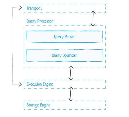
General DBMS Architecture Components and Neo4j’s Unique Approach
Transport: At the outset of any interaction with a database, a client query arrives through the transport subsystem which in turn hands it over to the query processor.
- Neo4j functions the the same way.
Query Processor: The query processor then parses the query for interpretation, validation and so on, after which the query optimizer (i.e. query planner) then takes charge, finding the most efficient way to process and retrieve the data.
- Neo4j in particular uses what they call the Cypher Query Planner, which like most query planners bases optimizations on internal statistics, indexes, constraints, data placement and more.
Execution Engine: The output from the query processor of any database system is the execution plan, which is a sequence of operations to be carried out. This execution plan is handed to the execution engine which performs and aggregates the results.
- Neo4j decomposes queries into discreet elements that it calls operators, which are combined into a tree-like structure (described in more detail below) which is the execution plan. Also in Neo4j the leaf node ultimately resolves to the record and the output is piped all the way up the tree, while non-leaf node requires the sub-selection output set from the upstream branches.
- TIP 1: For Neo4j performance tuning, to better understand the queries developers can use the Cypher EXPLAIN query to see the execution plan and the Cypher PROFILE query to track how the rows are passed through operators.
Database Indexing and Neo4j Index Performance
For DBMS systems, indexing is a crucial capability for improving read performance. As a refresher, a database index is a structure (e.g. much like the index of a book) that organizes data records on disk in a way that facilitates its retrieval, mapping record keys to the location on disk. But as a database grows so does the index, and over time that can impact particularly write performance (e.g. inserts, updates, deletes), and they can also take up significant amounts of disk space.
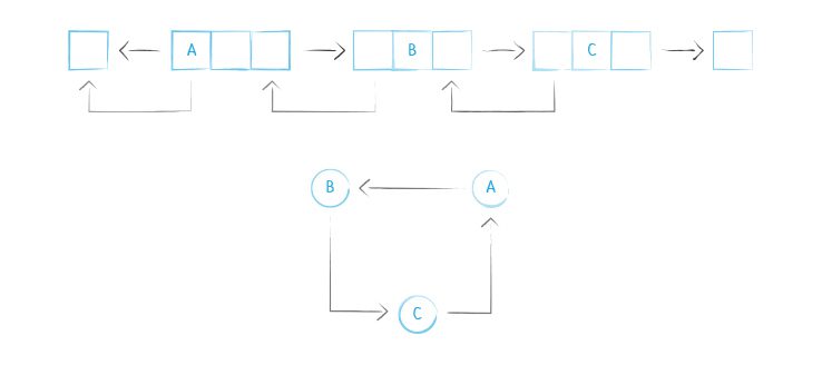
Neo4j index performance (or any native graph database) does not rely on traditional indexing which would have a significant negative impact on performance. It instead utilizes what is called index-free adjacency, which means that every node (which in Neo4j are only ever singly-linked lists) references its adjacent / next node directly, which functions as a kind of micro-index stored in the node itself. Edges in Neo4j are always doubly-linked lists referencing not only the next node but also the previous one.
Using this index-free adjacency is what actually defines native graph processing. It is also critical for high-performance graph queries since native graph queries and processing will thus perform at a constant rate regardless of data size (i.e. query times are always proportional to the amount of the graph being searched/the size of the traversal- “O(1)” vs the size of the graph “O(log n)“), as compared to using traditional indexing which takes longer as the data grows. The image below visually depicts a doubly-linked list for the edges in the graph and the adjacency where each node references neighbor node(s).
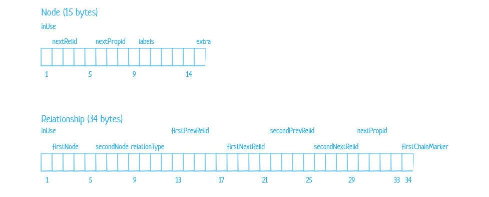
To dive even deeper, the below table illustrates how the bytes themselves are distributed for a node and how all the elements of that node are used by the index:
|
Byte | Description |
|
0 |
Used record or able to be reclaimed |
|
1-4 |
ID of the first relationship |
|
5-8 |
ID of the first property |
|
9-14 |
ID to the store label or inline label |
|
15 |
Reserved |
The image below shows the exact store file record structure for both nodes and relationships as use by the index as well:
Below are the steps Neo4j uses to perform a lookup and traversal of the graph:
- The lookup request moves the pointer to the first record in the global index
- It then computes in bytes the offset by multiplying the starting node (or other object) byte size or relationship ID byte size by the node store record size (also in bytes) to find the starting node address.
- It then also looks up the byte size address(es) for related edges and properties in the lookup request.
Looking at the file record structure figure above for relationships, we see that a graph relationship holds the address for the start node (first node), end node (second node), and related relationship and property blocks in the record structure, but in both directions (next and previous).
By referencing data in memory and directly by using pointers, and by iterating over linked lists of the various objects (e.g. nodes, edges, etc) moving from pointer to pointer (which is called “referencing” in Java, and what Neo4j often calls “chasing pointers”), it reduces the number of actual disk reads required of a query dramatically helping Neo4j performance.
Neo4j Global Index Types
Neo4j index performance is based on 3 different global registry index types that it provides: b-tree, full-text and token lookup for different use cases.
- B-tree indexes maps a property to a node or an edge, performing an exact index lookup on all types. B-tree indexes are one of the most popular storage structures, common to most other databases, and are known to provide efficient operations and use of hardware. They tend to reduce the tree height, also enabling ordered sequential access. In the context of Neo4j they are designed to map exact property value to a node or relationship enabling faster traversals.
- Token lookup indexes are now created by default for all node labels and relationship tyoes as of Neo4j 4.3. Often it is more performat to select and use an optimized b-tree index, but the token index is now always available by default. This index enables matching a node through its label which avoids scanning and filtering all the node labels. Tip 2: Despite associated performance gains for writes when dropping the token index, because the index is also used for improving efficiency in populating the other index options as well as improving read queries, it is worth taking time to consider keeping it.
- Full-text indexes are implemented for use cases involving text search (using Apache Lucene)
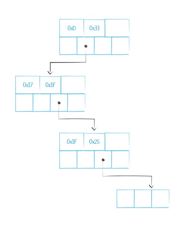
Below is a figure illustrating the structure of the B-tree index. One can see from the structure the singly-linked structure where the parent node points to a child node and so on down the tree (though not shown here, each node holds a key/value pair).
The indexing and lookup approaches described above are powerful for driving performance, but they must work in concert with a storage architecture that supports it. Next, we will look in detail at the other aspect of what makes a native graph database truly native- the storage engine.
Native Graph Storage Engine
The easiest way to sum up what a native graph storage engine is, would be that the storage structures are purpose-built for graph optimized interactions. In the case of Neo4j, this native graph storage is evidenced in the fixed record structure of nodes, edges, and so on, as well as the store files that contain the records, as explained below. For Neo4j, as with any database, there are two principal kinds of storage that it leverages, physical storage and memory (described in more detail further below).
Physical storage
In Neo4j, data stored on physical disk is stored according to the index-free adjacency principle. The graph is structured in a set of files known as store files that are generally broken down by record type (that contain the fixed-size record format described previously) as shown in the table below:
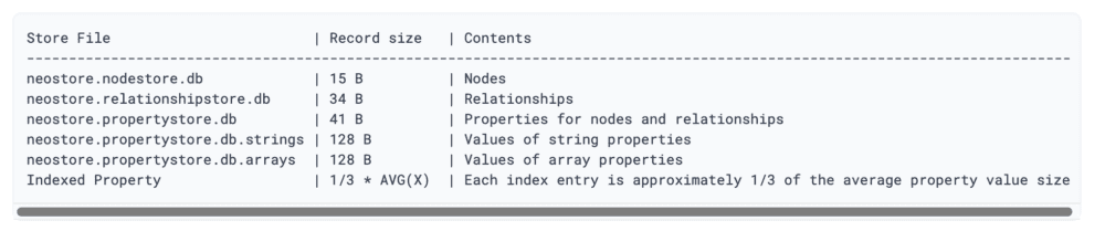
TIP 3: For Neo4j performance tuning, use EXT4 and XFS, and avoid NFS or NAS file systems.
TIP 4: Another Neo4j performance tuning option is to store data and transaction logs on separate drives to avoid contention and allow I/O to occur at the same time for both.
Memory
Neo4j uses a disk-based approach for data storage but also relies heavily on memory for caching disk contents for performance (or as temporary storage). As would be expected, Neo4j performs best when leveraging the data cached in-memory as much as possible as it significantly reduces the disk I/O expense.
Tip 5: Because Neo4j is Java-based, an additional option is to configure the object memory directly via the neo4j.conf file. In this way, developers can leverage the JVM to tune the memory configuration to maximize performance by balancing the JVM heap space with the garbage collector use, among other tuning options.
In effect though, and particularly as the cost of memory has come down so significantly in the last decade, it is now quite normal to store one’s entire graph in memory for production use.
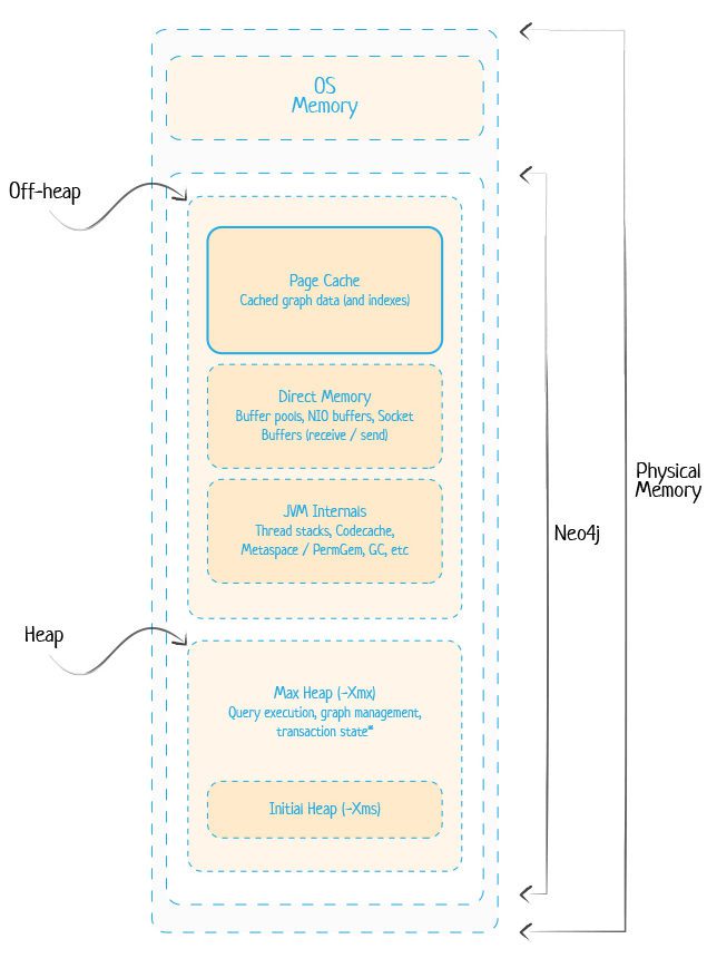
TIP 6: To adequately size Neo4j memory settings, here is a memory calculation rule of thumb: Total Physical Memory = Heap + Page Cache + OS Memory. One can also accurately calculate the required space for the core data since all the records are fixed size.
To become more familiar with Neo4j memory use, this figure below puts it in context:
Neo4j Performance through Hardware Scaling (Neo4j distributed)
Massive scalability is still a challenge for all graph databases and has been put forward as one of the limitations of neo4j, but as the market and technology matures Neo4j is solving the problem creatively and well. The main issue is the problem of maintaining state across many servers, to keep them synchronized while scaling, given the uniqueness of graph data as discussed below.
Until recently, Neo4j could only scale horizontally by using replication (copying one database content on multiple servers) and then using Neo4j sharding (to scale) through a workaround technique call cache sharding which routes each request to the database instance that holds the desired portion of the graph that is already in memory. Conversely, the standard approach to sharding distributes data on different cluster nodes, each of which is able to perform its own reads and writes, often with different users accessing duplicated, separate sets of data.
So why not just use the standard approach to sharding? The reason is found in the fact that the property graph model relies on nodes and the physical connections between them as the basis for queries. If a query must manage sub-graphs, across network boundaries and still attempt to maintain ACID compliance with all the relationships, data consistency, and integrity, it becomes a uniquely challenging problem to solve. In fact, the difficulty in solving this is so significant that it is classified in the NP-hard problems category.
Are there Neo4j Scalability Limits? Making Neo4j Sharding Work
So does this represent hard Neo4j scalability limits? Not at all. As of the release of its version 4.0, Neo4j is clearly now well on the path of offering a truly Neo4j distributed database approach, which also makes it more possible to approach standard sharding practices.
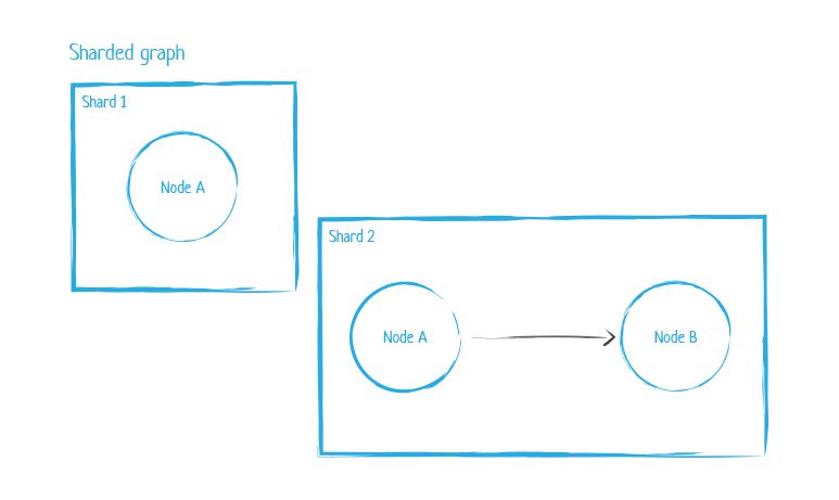
So how has the Neo4j approach to sharding evolved? As of version 4.0, Neo4j shards by spreading subgraphs across different Neo4j database instances across servers and even networks. To maintain the relationship between entities, it duplicates the node that holds the relationship between two shards, on both shards. What this means is that while now a developer can shard datasets, they still cannot shard the relationships since it is not possible to traverse shards at this point.
To manage the challenge of state across servers and networks, Neo4j now also provides Neo4j Fabric to manage the querying process. It can be thought of as a proxy that manages requests and connection information across all the shards by keeping a master representation of the database entities and locations, being aware of all shards at all times. Neo4j Fabric itself does not hold any data.
One of the challenges that still remain when sharding in general is the need to plan access patterns ahead of time since fallacies of distributed computing exist in this context as well. To effectively counter those risks Neo4j has offered causal clustering in order to drive consistency.
A causal cluster is designed to facilitate a single unit of servers (cluster) to maintain its state across replicas, even when communications may be interrupted. It provides a solution for synchronizing state across many servers while scaling by applying causal consistency and a consensus algorithm.
The causal consistency model defines cause and effect. That is, concurrent writes are applied in the same order that they occur by looking at the order causally related operations are processed (often called causal order). In this way, it ensures that you read-your-write for distributed consistency.
For the consensus algorithm, it also facilitates state agreement in a distributed context. To accomplish this, Neo4j leverages the Raft protocol to handle master election and maintain a consistent log across the cluster. This represents a significant step forward in being able to leverage ACID-compliant sharding in a distributed context. Check out this interactive presentation explaining the Raft protocol in more detail.
Are there Limitations of Neo4j?
As with all databases there are use cases that are best fit for each one. So in the sense that not every database use case is for graph, then the limitations of Neo4j are the same as every other database. Typically when this question comes up though, it is more about Neo4j scalability limits, and as the platform has matured this question is becoming moot. In fact, As of Neo4j 4.0 with the sharding issue well on its way to being creatively resolved, the combination of vertical and now horizontal scaling enable just about any graph use case, at any scale imaginable.
Neo4j Performance: Conclusion
By exploring the performance advantages of Neo4j’s native-graph architecture, it becomes evident that as a database system, Neo4j performance tuning is just part of the very architecture in many ways. There are some helpful tips included here, but look out for future articles on neo4j graph modeling and optimizing neo4j query design as additional ways to positively and more directly impact Neo4j performance.
Graphable helps you make sense of your data by delivering expert data analytics consulting, data engineering, custom dev and applied data science services.
We are known for operating ethically, communicating well, and delivering on-time. With hundreds of successful projects across most industries, we have deep expertise in Financial Services, Life Sciences, Security/Intelligence, Transportation/Logistics, HighTech, and many others.
Thriving in the most challenging data integration and data science contexts, Graphable drives your analytics, data engineering, custom dev and applied data science success. Contact us to learn more about how we can help, or book a demo today.
Still learning? Check out a few of our introductory articles to learn more:
- What is a Graph Database?
- What is Neo4j (Graph Database)?
- What Is Domo (Analytics)?
- What is Hume (GraphAware)?
Additional discovery:
- Hume consulting / Hume (GraphAware) Platform
- Neo4j consulting / Graph database
- Domo consulting / Analytics - BI
We would also be happy to learn more about your current project and share how we might be able to help. Schedule a consultation with us today. We can also discuss pricing on these initial calls, including Neo4j pricing and Domo pricing. We look forward to speaking with you!
Graphable helps you make sense of your data by delivering expert analytics, data engineering, custom dev and applied data science services.
We are known for operating ethically, communicating well, and delivering on-time. With hundreds of successful projects across most industries, we have deep expertise in Financial Services, Life Sciences, Security/Intelligence, Transportation/Logistics, HighTech, and many others.
Thriving in the most challenging data integration and data science contexts, Graphable drives your analytics, data engineering, custom dev and applied data science success. Contact us to learn more about how we can help, or book a demo today.
We are known for operating ethically, communicating well, and delivering on-time. With hundreds of successful projects across most industries, we thrive in the most challenging data integration and data science contexts, driving analytics success.
Contact us for more information: